Introduction to Pipelining and Shell Review

Overview

Questions

• How can I interact with computer commands fully automatically?

Objectives

• Explain the advantages of pipelining.
• Write simple shell scripts to explore directories, remove files, read and write text files, and execute Python scripts.

Automation and pipelining

---

Background

Humans and computers commonly interact in many different ways, such as through a keyboard and mouse, touch screen interfaces, or using speech recognition systems. The most widely used way to interact with personal computers is called a graphical user interface (GUI). With a GUI, we give instructions by clicking a mouse and using menu-driven interactions.

While the visual aid of a GUI makes it intuitive to learn, this way of delivering instructions to a computer scales very poorly. Imagine the following task: for a literature search, you have to copy the third line of one thousand text files in one thousand different directories and paste it into a single file. Using a GUI, you would not only be clicking at your desk for several hours, but you could potentially also commit an error in the process of completing this repetitive task. This is where we take advantage of the Unix shell. The Unix shell is both a command-line interface (CLI) and a scripting language, allowing such repetitive tasks to be done automatically and fast. With the proper commands, the shell can repeat tasks with or without some modification as many times as we want. Using the shell, the task in the literature example can be accomplished in seconds.

The Shell

The shell is a program where users can type commands. With the shell, it’s possible to invoke complicated programs like climate modeling software or simple commands that create an empty directory with only one line of code. The most popular Unix shell is Bash (the Bourne Again SHell — so-called because it’s derived from a shell written by Stephen Bourne). Bash is the default shell on most modern implementations of Unix and in most packages that provide Unix-like tools for Windows. Note that ‘Git Bash’ is a piece of software that enables Windows users to use a Bash like interface when interacting with Git.

Using the shell will take some effort and some time to learn. While a GUI presents you with choices to select, CLI choices are not automatically presented to you, so you must learn a few commands like new vocabulary in a language you’re studying. However, unlike a spoken language, a small number of “words” (i.e. commands) gets you a long way, and we’ll cover those essential few today.

The grammar of a shell allows you to combine existing tools into powerful pipelines and handle large volumes of data automatically. Sequences of commands can be written into a script, improving the reproducibility of workflows.

In addition, the command line is often the easiest way to interact with remote machines and supercomputers. Familiarity with the shell is near essential to run a variety of specialized tools and resources including high-performance computing systems. As clusters and cloud computing systems become more popular for scientific data crunching, being able to interact with the shell is becoming a necessary skill. We can build on the command-line skills covered here to tackle a wide range of scientific questions and computational challenges.

Let’s get started.

When the shell is first opened, you are presented with a prompt, indicating that the shell is waiting for input.

BASH

$

The shell typically uses $ as the prompt, but may use a different symbol. In the examples for this lesson, we’ll show the prompt as $. Most importantly, do not type the prompt when typing commands. Only type the command that follows the prompt. This rule applies both in these lessons and in lessons from other sources. Also note that after you type a command, you have to press the Enter key to execute it.

The prompt is followed by a text cursor, a character that indicates the position where your typing will appear. The cursor is usually a flashing or solid block, but it can also be an underscore or a pipe. You may have seen it in a text editor program, for example.

Note that your prompt might look a little different. In particular, most popular shell environments by default put your user name and the host name before the $. Such a prompt might look like, e.g.:

BASH

nelle@localhost $

The prompt might even include more than this. Do not worry if your prompt is not just a short $. This lesson does not depend on this additional information and it should also not get in your way. The only important item to focus on is the $ character itself and we will see later why.

Exploring directories

So let’s try our first command, ls, which is short for listing. This command will list the contents of the current directory:

BASH

$ ls

OUTPUT

Desktop     Downloads   Movies      Pictures
Documents   Library     Music       Public

If you saw something like the above output, then you are in the root directory of your computer. We want to navigate to make-lesson instead. So let’s use the command cd. The format is cd followed by a directory name to change our working directory. cd stands for ‘change directory’, which is a bit misleading. The command doesn’t change the directory; it changes the shell’s current working directory. In other words it changes the shell’s settings for what directory we are in. The cd command is akin to double-clicking a folder in a graphical interface to get into that folder.

Let’s try this out! For example, on a Windows computer, the typical path to the directory looks like this:

BASH

$ cd C:/Users/Your_name/Documents/make-lesson

Note that if you use Windows, you should ensure that you use forward slashes instead of backward slashes, which are the normal slash in Windows. If you use Mac, then you normally use forward slashes anyways.

These commands will move us to the right directory. You will notice that cd doesn’t print anything. This is normal. Many shell commands will not output anything to the screen when successfully executed. But if we run pwd after it, we can see that we are now in the right directory.

If we run ls -F without arguments now, it lists the contents of our directory for this workshop, because that’s where we now are:

BASH

$ pwd

OUTPUT

C:/Users/Your_name/Documents/make-lesson

BASH

$ ls -F

OUTPUT

books/  countwords.py*  plotcounts.py*  testzipf.py*

File handling

---

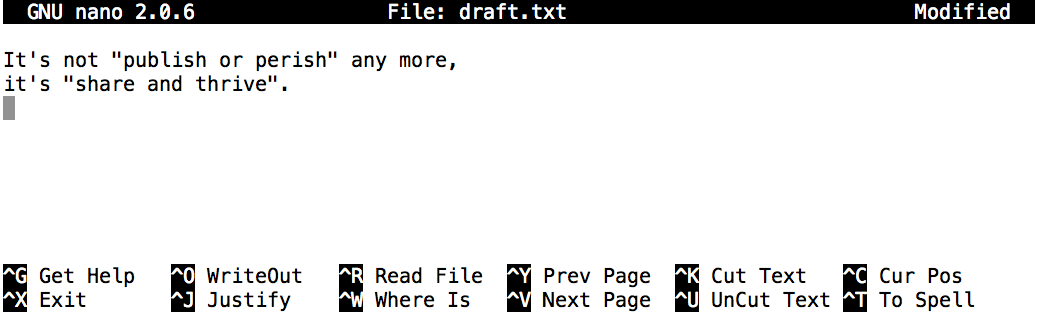
Let’s run a text editor called Nano to create a file called newbook.txt:

BASH

$ nano books/newbook.txt

Let’s type in a few lines of text.

Once we’re happy with our text, we can press Ctrl+O (press the Ctrl or Control key and, while holding it down, press the O key) to write our data to disk. We will be asked to provide a name for the file that will contain our text. Press Return to accept the suggested default of newbook.txt.

Once our file is saved, we can use Ctrl+X to quit the editor and return to the shell.

nano doesn’t leave any output on the screen after it exits, but ls now shows that we have created a file called draft.txt:

BASH

$ ls books

OUTPUT

abyss.txt  isles.txt  last.txt  LICENSE_TEXTS.md  newbook.txt  sierra.txt

Now if you want to view your glorious creation any time, you can use the head command to see the beginning of the book:

BASH

$ head books/newbook.txt

OUTPUT

It's not "publish or perish" any more,
it's "share and thrive".

Our book needs a more glorious filename than just newbook.txt. So we can go ahead and use the mv (‘move’) command to change its filename to coolbook.txt:

BASH

$ mv books/newbook.txt books/coolbook.txt

On second thoughts, adding our own book to the corpus (however short) was probably not the smartest idea, so let’s delete it using the rm (‘remove’) command:

BASH

$ rm books/coolbook.txt

Counting words

---

Zipf’s Law

The most frequently-occurring word occurs approximately twice as often as the second most frequent word. This is Zipf’s Law.

We’ve compiled our raw data i.e. the books we want to analyze and have prepared several Python scripts that together make up our analysis pipeline.

Let’s take quick look at one of the books using the command head books/isles.txt.

Our directory has the Python scripts and data files we will be working with:

OUTPUT

|- books
|  |- abyss.txt
|  |- isles.txt
|  |- last.txt
|  |- LICENSE_TEXTS.md
|  |- sierra.txt
|- plotcounts.py
|- countwords.py
|- testzipf.py

The first step is to count the frequency of each word in a book. For this purpose we will use a Python script countwords.py. We will run this Python script on the command line, rather than running it inside an environment like JupyterLab or VSCode. This is achieved by writing the if __name__ == '__main__': statement inside Python scripts; for example, countwords.py has the following code at the bottom:

PYTHON

if __name__ == '__main__':
    input_file = sys.argv[1]
    output_file = sys.argv[2]
    min_length = 1
    if len(sys.argv) > 3:
        min_length = int(sys.argv[3])
    word_count(input_file, output_file, min_length)

This script takes two command line arguments. The first argument is the input file (books/isles.txt) and the second is the output file that is generated (here isles.dat) by processing the input.

We can run countwords.py in the Bash shell by typing python, then the name of the script, then the names of the input and output files.

BASH

$ python countwords.py books/isles.txt isles.dat

Let’s take a quick peek at the result.

BASH

$ head -5 isles.dat

This shows us the top 5 lines in the output file:

OUTPUT

the 3822 6.7371760973
of 2460 4.33632998414
and 1723 3.03719372466
to 1479 2.60708619778
a 1308 2.30565838181

We can see that the file consists of one row per word. Each row shows the word itself, the number of occurrences of that word, and the number of occurrences as a percentage of the total number of words in the text file.

We can do the same thing for a different book:

BASH

$ python countwords.py books/abyss.txt abyss.dat
$ head -5 abyss.dat

OUTPUT

the 4044 6.35449402891
and 2807 4.41074795726
of 1907 2.99654305468
a 1594 2.50471401634
to 1515 2.38057825267

Let’s visualize the results. The script plotcounts.py reads in a data file and plots the 10 most frequently occurring words as a text-based bar plot:

BASH

$ python plotcounts.py isles.dat ascii

OUTPUT

the   ########################################################################
of    ##############################################
and   ################################
to    ############################
a     #########################
in    ###################
is    #################
that  ############
by    ###########
it    ###########

plotcounts.py can also show the plot graphically:

BASH

$ python plotcounts.py isles.dat show

Close the window to exit the plot.

plotcounts.py can also create the plot as an image file (e.g. a PNG file):

BASH

$ python plotcounts.py isles.dat isles.png

Finally, let’s test Zipf’s law for these books:

BASH

$ python testzipf.py abyss.dat isles.dat

OUTPUT

Book	First	Second	Ratio
abyss	4044	2807	1.44
isles	3822	2460	1.55

So we’re not too far off from Zipf’s law.

Key Points

• Shell scripts allow us to handle file systems and run Python scripts from the command line.